A practical comparison of GeoTIFF compression algorithms
Not all GeoTIFFs are alike. Two images with identical information might have a different format for storing the data.
Working with earth observation data invariably means working with GeoTIFF files. It is without question the most common way of handling and delivering georeferenced raster data. But not all GeoTIFFs are alike. Two images with identical information might have a different format for storing the data.
Bandwidth is expensive, and always limited in the end, so it's a good idea to minimize the file sizes without losing information. Let's take a practical look at different ways to store the data using common lossless compression methods available.
Input
For testing, we will use a raw version of a Terramonitor Sentinel Mosaic product. The file is available for download for anyone with a Terramonitor account. The input consists of
- a GeoTIFF with 10 meter Sentinel-2 bands (4 bands)
- a GeoTIFF with 20 meter Sentinel-2 bands (6 bands)
- a GeoTIFF with calculated NDVI, stored as an integer (1 band)
All data was handled as unsigned 16-bit integer.
Test suite
Our test suite creates three files of each of the input files
- a file with just the compression applied
- a file with compression and internal tiling – this format is also called "cloud optimized GeoTIFF"
- a file with compression, internal tiling and overview files, for quicker previews in GIS software
Adding internal tiling and overviews produces a so called "Cloud Optimized GeoTIFF". At Terramonitor, we serve all our data from the cloud, and we definitely want our GeoTIFF files to be cloud optimized!
All the output files were produced using gdal_translate from GDAL 2.4.2 with appropriate flags -co COMPRESS=LZW and/or -co TILED=YES, et cetera.
No compression
The base case is not applying any compression to the files. This is a relatively quick operation that only took 10 seconds to run on the test machine, and serves as a baseline.
|input|uncomp.| uncomp. + tiling| uncomp. + tiling + ovs|
|:--:|--:|--:|--:|--:|
|10m|796|818|1093|
|20m|298|315|420|
|ndvi|199|204|273|
Table. File sizes in megabytes when no compression is applied
We see here that while adding internal tiling adds a modest 3-6% increase in file size, adding the overviews causes the file size to increase by 40%! Next, let's see how our compression algorithms deal with that.
LZW
Lemper-Ziv-Welch (LZW) may be considered the go-to compression algorithm for GeoTIFF files. It is relatively fast and gives fairly good compression. Running the test suite took a few seconds shy of a minute. We ran it without predictors.
|input|comp.| comp. + tiling| comp. + tiling + ovs|
|:--:|--:|--:|--:|--:|
|10m|719|705|942|
|20m|324|322|430|
|ndvi|139|132|178|
Table. File sizes in megabytes when LZW is applied
The compression algorithm in fact benefits from internal tiling as the data is ordered so that tiles with similar data are organized next to each other in the file. Alas, adding the overviews still causes a 30±2% increase in file size. Compared to the uncompressed file sizes, the benefits are anything from a 35% reduction in file size with the NDVI input, to an appalling 2% increase in the case of 20-meter bands.
DEFLATE
Deflate is most likely the second compression algorithm you will find. It generally provides better results than LZW, but is slower: in this case the test suite ran for 2,5 minutes, over twice slower than LZW. We ran it with the default parameters: zlevel 6, no predictors.
|input|comp.| comp. + tiling| comp. + tiling + ovs|
|:--:|--:|--:|--:|--:|
|10m|606|590|790|
|20m|244|242|323|
|ndvi|123|113|154|
Table. File sizes in megabytes when DEFLATE is applied
Again, internal tiling is beneficial for compression, but adding overviews adds a very similar 28±4% increase in file size. Compared to the uncompressed files, applying Deflate shaves from 23 to 27 percent of bytes in the case of regular rasters, and up to 44% reduction in file size in the optimal case.
ZSTD
The newest algorithm of the three, Zstandard (zstd) was developed as recently as 2016. It is the slowest, and the test suite took 3,5 minutes to complete. We ran it with the default zstd level of 9.
|input|comp.| comp. + tiling| comp. + tiling + ovs|
|:--:|--:|--:|--:|--:|
|10m|607|557|754|
|20m|248|237|319|
|ndvi|121|109|149|
Table. File sizes in megabytes when ZSTD is applied
The file sizes are extremely similar to the ones produced with Deflate. Even the largest difference (10m bands, compression, tiling and overviews) is under 5%. While ZSTD provides the best results in terms of file size, it took noticeably longer to run than Deflate.
Summary
Setting a time limit and tuning the compression levels of ZSTD and Deflate might very well produce the same results, so it's hard to say which one is best suited for a specific purpose.
Below is a summary of the compression ratios of each method in the worst case: 10-meter Sentinel-2 bands, internal tiling and overviews.
| Method | Compression ratio | Reasons to use |
|---|---|---|
| LZW | 1.16:1 | Quick to run and easy to adopt |
| DEFLATE | 1.38:1 | A slower but better performing alternative to LZW |
| ZSTD | 1.45:1 | Promising, CPU intensive but not mature |
Table. Summary of the results of the different compression algorithms
Further reading
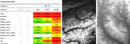
For an in-depth comparison of the compression algorithms presented here and a few more, see this post by Koko Alberti:
If you are interested in how well our compression algorithms work in practice, please get acquainted with our Analysis Ready products.

